Today is our last lab and we are going to end by applying some computational algorithms to words.
Your reading for today was a blog post by Ted Underwood talking about the ways text analysis can be used in humanities research. Key point: Text mining is, at the root, counting words and identifying patterns in the ways words are used. What are the different ways Underwood identifies that we can use our word counts?
In Box, I have uploaded a collection of word documents for us to explore, stored in the “Camping” folder inside of “Data.” These were written by the late Harold Camping, who predicted the end of the world in 2011 (and previously in 1994). Download these files to your local machine.(https://alabama.box.com/s/k8311tewq4zeez7t3p3pqc1m42a3a90z)
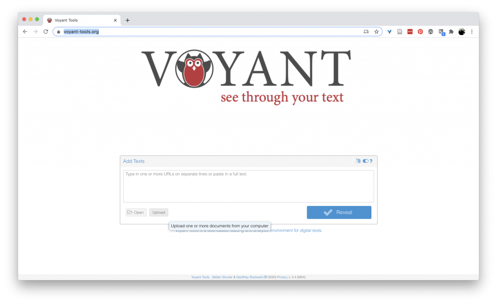
We are going to experiment with a browser-based text analysis tool today: Voyant-tools.
Navigate to https://voyant-tools.org/ and select the “upload” button.
Select all four word documents from the “Camping” folder and click “Open.”
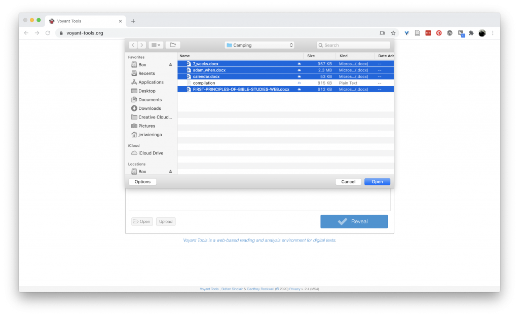
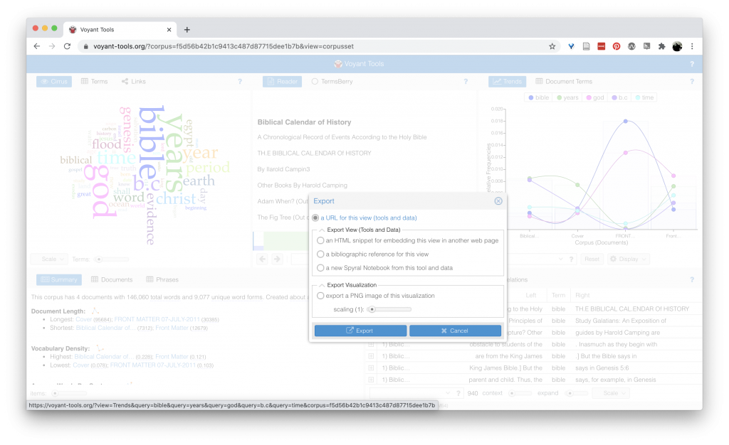
This loads the documents into Voyant’s system where it counts up the words used in each document, performs a number of computations, and then presents that information in 5 different grids.
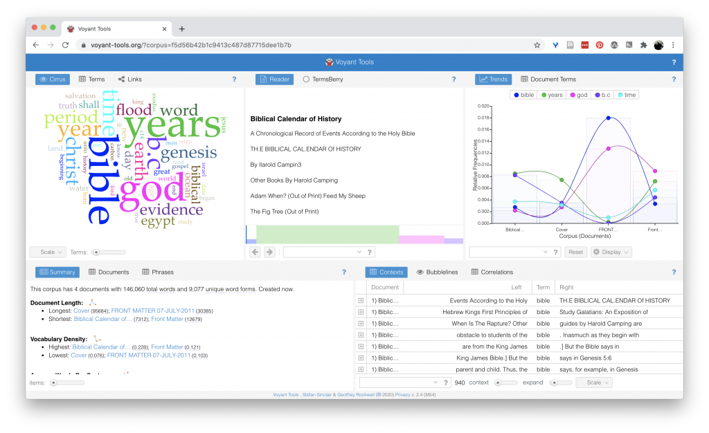
Starting at the top left corner and working across, left to right:
First, we have a word cloud. Ah word clouds. We all thought we were so cool in the early 2010 with our word clouds. A word cloud represents the most common words in the corpus or document, sized according to how frequently the word occurs. At the bottom of this grid, you can control how many words to include in the cloud, as well as whether the cloud is made up of the whole corpus or individual documents (and which one.) Try out a few of the settings to get a feel of how this visualization works.
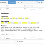 Next, we have a “Terms” option across the top of the grid. This gives us a table view of the most common words in the documents, and a chart of the relative frequency (how frequent the word is in each individual document.) This lets us see if a word is common across all the documents or if it is particularly significant in one document. Additionally, the [+] at the far left column expands the information about the word, showing the distribution of the word (over what is undefined …), collocates (words that appear with the target word), correlations (words whose frequencies trend together), and phrases (a snippet of a word in context).
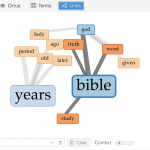 Finally, “Links” gives us our keywords in blue and the words that occur with that keyword in orange, connected with lines, with the width of the line showing the strength of the connection between the words. You can choose other words from the drop down at the bottom of the box.
So, which of the different forms of text analysis that Underwood identified are going on in here? Looking at these words, do you have any questions about how things are being counted?
 The second grid gives us a view of the documents, and hovering over individual words shows the frequency of that word in the document. Clicking a word will update the grid to the right to show the frequency of the word over all the documents in the corpus. It also activates a line inside the map at the bottom of the grid showing the presence of the word over each document.
The second grid also has a “TermsBerry” grid, which reveals top terms, the relationship between terms, and the number of books the term appears in. ( This one has a lot going on, which makes it hard to use.)
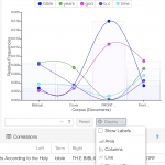 The third grid shows the relative frequency of select words in each of the documents. There are options for how this data is displayed at the bottom of the grid. Toggle through these. What do these visualizations communicate well? What is unclear?
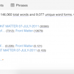 Down to the second row, left side of the dashboard, we have have a summary of the documents being analyzed, including total words, total unique words (what is a word anyways), vocabulary density or percentage of unique words), and most distinctive words for each text.
Where do these connect to Underwood’s taxonomy of text analysis?
 The final grid provides a window onto contexts of words. This format, also called “key words in contexts” or KWIC, provides the window of words before and after the target word. Clicking the [+] button provides an even wider context.
The bubblelines graph uses circle size to show the density of words at different points across the document. This can be useful for narrowing in on where a word is prevalent, or where it is an outlier.
And finally, a chart that attempts to compute the correlation strength between words. Correlation values range between 1 (strongly trend together) and -1 (strongly trend apart), with “significance” offering a “p-value” or the probability that the correlation is due to the null hypothesis (that there no correlation, or the word distribution is random).
All that from counting words.
But wait, there is more!
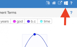 In the upper right corner, there is a menu that appears when you hover (an interesting design choice). Click the “windows” icon (4th one from the left). This gives you a whole list of additional ways to examine your documents. Each tool has a small explanatory text that you can access by hover over the “?” sign. (I thought I could walk you through them, but there are too many.) Explore one or two. If you find one that is particularly interesting, share back to the group.
You can export an individual view by clicking the outbound arrow in the top, hover activated, menu (first on the left). Depending on the took, you have one or two export options: “Export View” and “Export Visualization.” The visualization is a PNG image of the visualization. The view options let you export an HTML snippet to embed your visualization in a website.
Homework
For your final lab homework, explore 2-3 more text visualization tools and embed your results in a blog post. Write a brief description of why you choose that tool, what patterns it reveals about the text(s), and what additional questions it raises. Try to use a textual source connected to your research question (but if you cannot find one, you can use the Camping texts from class.)