Today we are going to work through two different ways to create data: combining existing data and constructing data from unstructured sources.
A third method is to create new data through the use of surveys or methods such as ethnography, oral history, or narrative inquiry. This is beyond our scope, but you can learn these techniques from a variety of disciplines, including history, anthropology, and religious studies.
Chapters 4 and 5 of Prepare Your Data for Tableau cover combining data in greater detail. Use these as a resource as you work on your homework.
But first off – we are going to switch over to the county-level data from the ARDA. This is the same data — all of your reading and our conversations about the data still apply. But the county-level does not have the compiling errors that we discussed in the state-level data. Because it is a large file, we are going to limit the data to the state of Alabama for class.
So to start, let’s load up the ARDA data in Tableau.
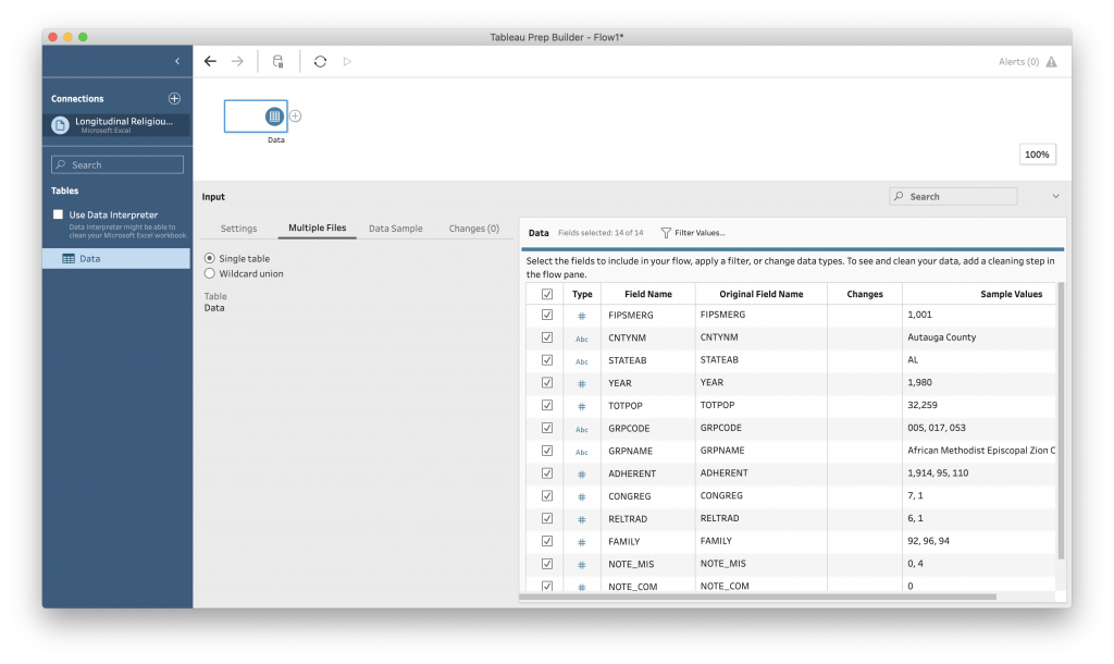
The fields are roughly the same as in the State file, with the addition of county information.
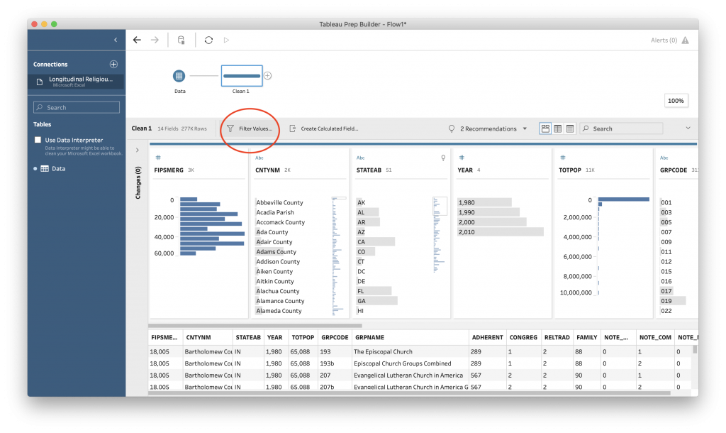
Add a cleaning step. You may notice that Tableau takes a lot longer to load up the data than it did with the State file. This is because this is a much bigger data file than the State file, as there are rows for a large percentage of the counties in each state. Grab a cup of tea while the data loads.
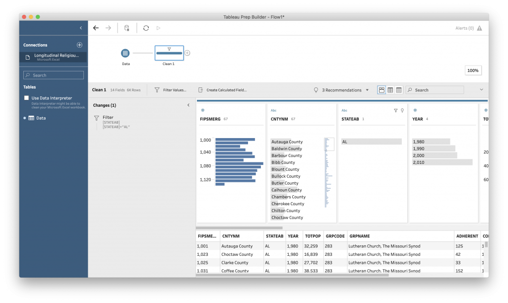
First, let’s filter the data to the state of Alabama.
This brings you to a rather strange blank box.
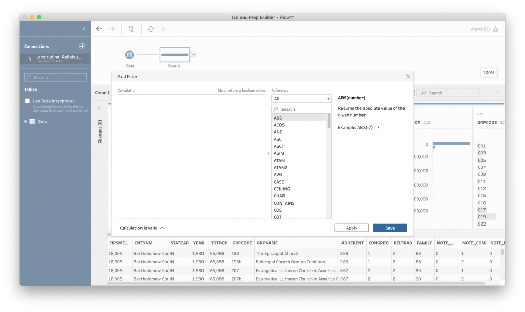
This interface is one of the places in Tableau where you need to think a little bit like a programmer. By that I mean, you need to think in terms of functions. For the filter, we want all of the rows where “State” is AL. To do that, the syntax is [fieldname]=”value we want”. The column name goes inside brackets ([ ]), and the value we want goes inside “” because it is a string. (“string” is another programming word to mean word or group of words. Think “string of letters”.)
So … we want our search box to read:
[STATEAB]="AL"
The filter is case-sensitive, so be sure you enter the field name and the values exactly as they appear in the data. Computers are very literal, even in fancy visual programs like Tableau.
Select “Save” to apply the filter. “AL” is now the only value under “STATEAB”. You can see your work by clicking the arrow on the left side of the screen.
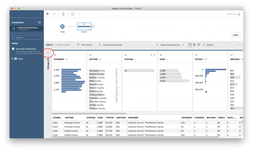
This will show you all of the changes you have made to the data. You can also modify or delete a change.
Combining Data
Now that we have the data narrowed down, we can start to combine it with other data.
First, let’s expand some of the fields that are currently coded as numbers. I created a google spreadsheet for the information in the codebook. Save a copy to your google drive.
Tableau is able to connect directly to google. To load the data, click the plus sign by “Connections” and choose Google Drive under “To a Server.” Authenticate and select the “Expanded Field Names” File.
You will now notice 5 tables listed in the blue sidebar.
Grab “RELTRAD” and drop it onto the Tableau canvas. This table gives the value assigned to the “Religious Tradition” code. To better preview the data, add a cleaning step to the RELTRAD data.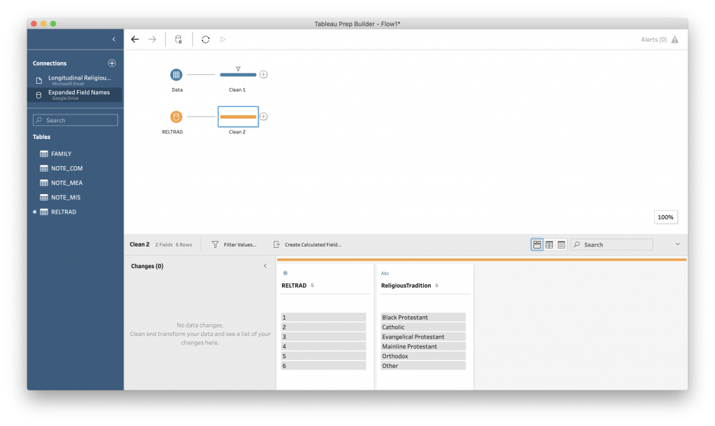
Now, to connect the two data tables, grab the Clean2 box and drag it up to the blue Clean 1 box. You should see two options appear: a “union” box under “Clean 1” and a “join” box to the right.
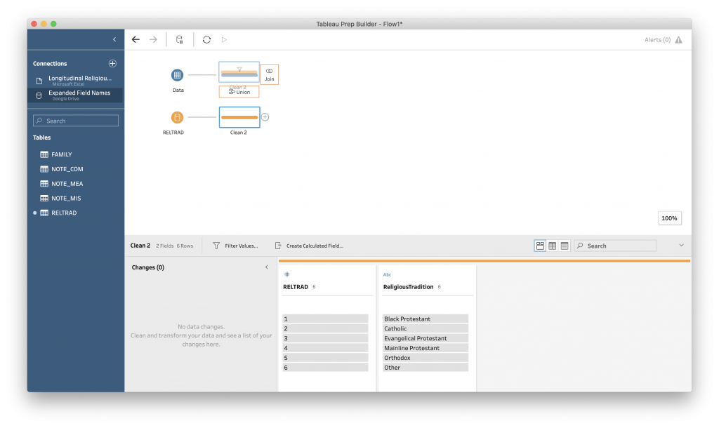
Here Tableau is showing to you visually what these two options will do. A union will attach the new data to the end of the first data file, making it longer. A join will combine the data in each row, based on a “key.” This makes the data wider, because you are adding more detail to each observation.
Because we are looking to expand the “RELTRAD” field with the spelled out “Religious Tradition,” we want a join.
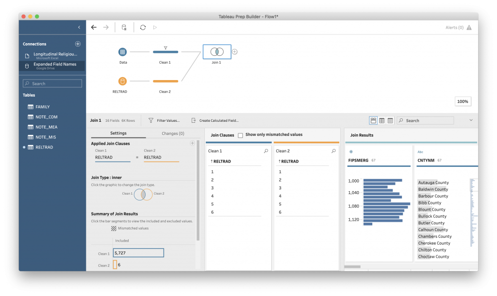
Tableau will make a guess about which fields to match. This is easiest when a field has the same name, as is the case here. We are telling Tableau that RELTRAD in the original data and RELTRAD in our expanded fields data are the same and, for each row in the original data, to add the information in the expanded fields data based on the number in the RELTRAD field.
Add a “Clean Step” to “Join 1” to see our new data file.
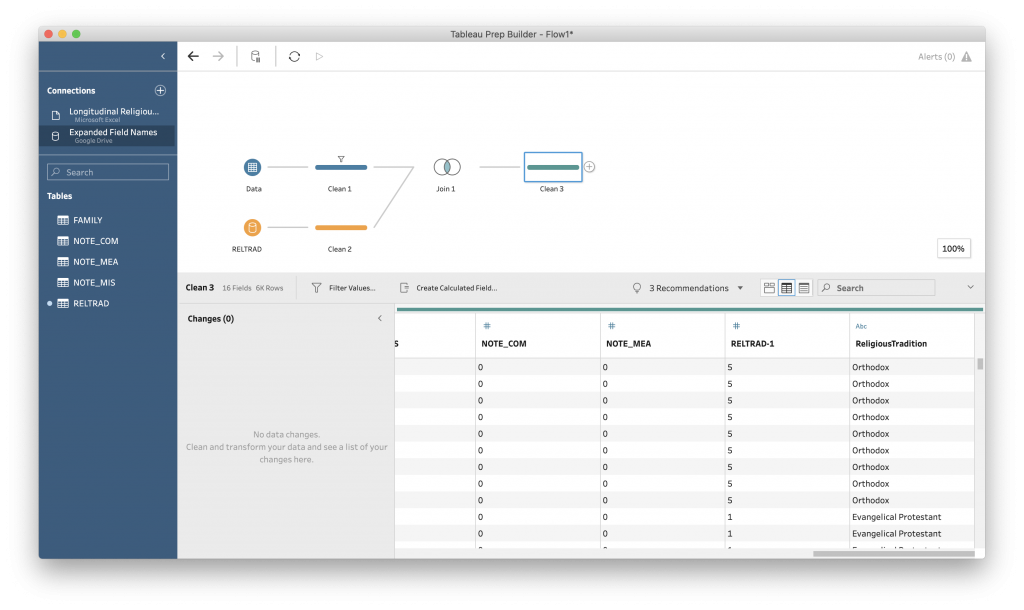
The data should look mostly the same, but with two new columns: RELTRAD-1 and “ReligiousTradition.”
The first few times you do a join successfully, it sort of feels like magic.
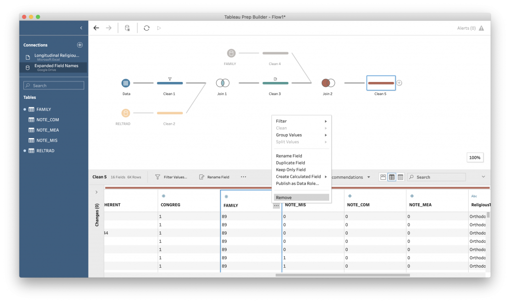
We can drop the RELTRAD and RELTRAD-1 columns, because we now have that information expanded. Mouse over the column head and click on the three dots that appear. Select “Remove” from the drop-down menu.
Few more things to mention – this interface gives us a lot of information about what is happening with the join, including whether any rows are being dropped. Here every row had RELTRAD information, so there are no “mismatched values” to worry about. Our join was a success.
This type of connection is called an “inner join” and is visualized in Tableau as the overlap between two circles. The resulting data will only include those rows that occur in both datasets. You use this join when you want where two datasets overlaps. One consequence of this is that any rows that don’t have the value you are matching on. We can see this in action with the FAMILY table.
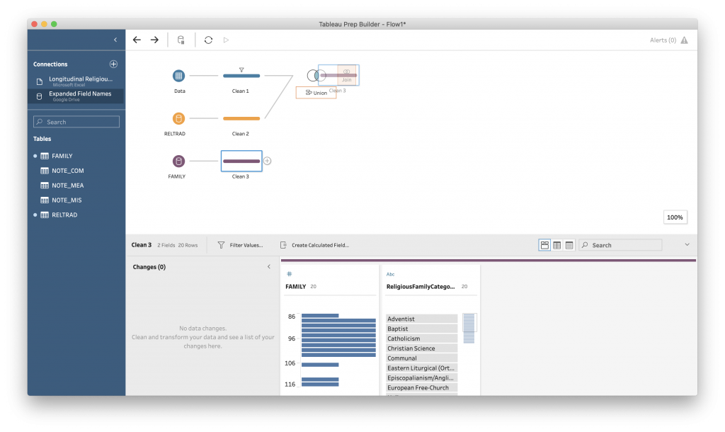
Grab the FAMILY table and drop it onto the Tableau canvas. Remember that there were “null” values under the FAMILY variable in our main dataset (this is still the case in the county data).
You can add a clean step to see the data, then drag your “Clean 4” box up and “join” it with “Clean 3” from your Join.
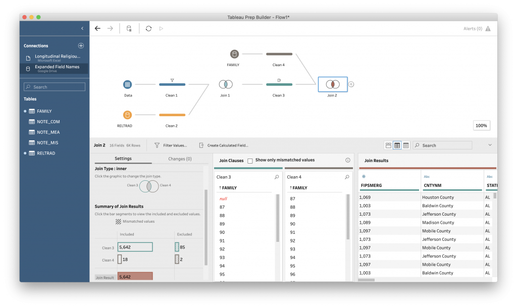
Looking at the “Summary of Join Results,” we can see that there are 85 rows in the original dataset and 2 in the FAMILY dataset that have been excluded on the Inner join.
But what if we don’t want to drop the 85 rows in the original dataset? This is where different types of joins come into play.
Tableau makes it easy for us to experiment with different join types using the Venn diagram under “Join Type.” What if we wanted to keep all of the data in the FAMILY table? Click on the “Clean 4” circle. This is a right join. There are now 0 rows excluded from the “Clean 4” data, but still 85 excluded from “Clean 3”. In addition, there are now 2 “unmatched” rows in the final data.
Right joins, and its pair left joins, let us designate one of the data sources as primary and one as supplemental. Of these, you are most likely to use the Left join, where your primary data is listed first and you pull in the information from the new data that has a match in your original data.
Let’s try a left join on our data. Click on the “Clean 4” circle again to de-select it and then click on the “Clean 3” circle.
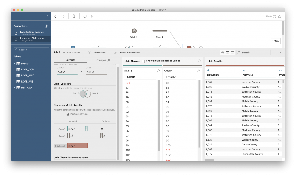
Now we have no rows excluded from the original data (good), and 85 unmatched rows, or rows with no FAMILY information, and two rows excluded from the expanded family name table.
Does this match what you would expect given our data?
(Note: you may want to give your cleaning steps more descriptive names …)
To finish up, let’s add a cleaning step to this second join to remove the original FAMILY fields.
Our final step here is to save our work. There are two aspects to consider here: the final output and the process you’ve created to get here – referred to in Tableau as a “flow.” Tableau Prep has its own format for saving the local data inputs, the process, and the resulting data. You can create this by going to “File” and “Save” in the Tableau menu. This file only works in Tableau Prep, however, so we need to export our final data into another format for use in Tableau Desktop or any other graphing library.
To do that, add a final “Output” step to your “flow.”
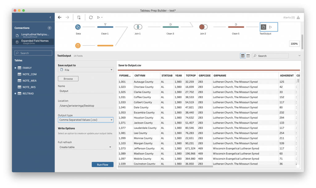
Select where you want to save your file. Then under “Output types” select your format. You have three choices:
- Tableau Data Extract (.hyper) for Tableau Desktop version 10.5 and later.
- Tableau Data Extract (.tde) for Tableau Desktop version 10.0 through 10.4.
- Comma Separated Values (.csv) if you want to share with someone who isn’t using Tableau.
Of these, .csv is going to be your most stable and multifunctional. But you can also choose .hyper for this class, as we are working in the most recent version of Tableau Desktop.
And finally, “Run Flow.” Tableau will work through all of the steps in your data, from loading the data files through to the last cleaning step, and generate the final output.
[ Take a Break]
Creating Data from Unstructured Data
Combining existing data sets will get you a long way toward having data that you can use to answer your questions.
But some times there is not an already existing dataset, or the data that does exist is not in a structured format. That is when you get to dive into the interpretive work of data creation.
Here I am going to use an example from my own research. This isn’t connected to religion in Alabama between 1980 and 2010, but it is useful conversation partner for exploring the challenges of creating data from historical documents.
Starting in the 1880s, the Seventh-day Adventist church produced annual Yearbooks that provided information on the church leadership, denomination-sponsored organizations, and the like. We are going to work with the SDA Yearbook from 1885.
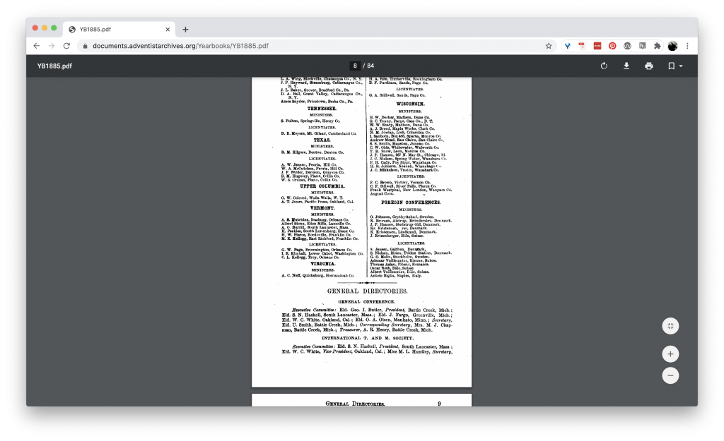
The Yearbook contains data, but it is structured for a human reader, not for a computer. The page scans that make up the PDF have been OCRed, meaning that the text has been recognized, but Tableau cannot make enough sense of the information to make it useful.
So, how do we go about turning this information into data? Keep the principles of Tidy Data in mind as your brainstorm.
…
…
…
Let’s start by describing the document as a whole. In terms of types of data, it is a published textual source, something that is known and can be linked to other published texts. So we will use a standard metadata scheme to describe it – Dublin Core.
We are going to be working in a Google Spreadsheet for this work. I have narrowed down the list of available variables to ones better suited for a textual resources such as this. Using the PDF and descriptions of the fields from Dublin Core, let’s fill out as many as we can.
…
…
To transcribe the information inside the PDF, we need to think through how best to organize. Remember from our Tidy Data reading that each type of observation should be organized in its own table.
Let’s create a new tab for the “Ministers” information.
What are our variable names? Is there any supporting information we might need for using this data as part of research?
Homework
For your lab homework, create a new tab in the SDA_Yearbook_1885 Google Sheet for some aspect of the information in the yearbook. Create a schema for the information (the variables) and fill out at least 10 rows.
On your blog, write a short blog post where you describe what you identified as an observation type and the schema you developed to organize the information into data. Explain why you chose to organize the information in that way. Be sure to identify which tab is yours.